Pathfinder Phase Workshop: Visualising Data

Description & purpose: This Notebook is designed to showcase the functionality of the Earth Observation Data Hub (EODH) as the project approaches the end of the Pathfinder Phase. It provides a snapshot of the Hub, the pyeodh API client and the various datasets as of February 2025.

Author(s): Alastair Graham, Dusan Figala, James Hinton, Daniel Westwood

Date created: 2025-02-18

Date last modified: 2025-02-25

Licence: This notebook is licensed under Creative Commons Attribution-ShareAlike 4.0 International. The code is released using the BSD-2-Clause license.

Copyright (c) , All rights reserved.

Redistribution and use in source and binary forms, with or without modification, are permitted provided that the following conditions are met:

Redistributions of source code must retain the above copyright notice, this list of conditions and the following disclaimer. Redistributions in binary form must reproduce the above copyright notice, this list of conditions and the following disclaimer in the documentation and/or other materials provided with the distribution. THIS SOFTWARE IS PROVIDED BY THE COPYRIGHT HOLDERS AND CONTRIBUTORS “AS IS” AND ANY EXPRESS OR IMPLIED WARRANTIES, INCLUDING, BUT NOT LIMITED TO, THE IMPLIED WARRANTIES OF MERCHANTABILITY AND FITNESS FOR A PARTICULAR PURPOSE ARE DISCLAIMED. IN NO EVENT SHALL THE COPYRIGHT HOLDER OR CONTRIBUTORS BE LIABLE FOR ANY DIRECT, INDIRECT, INCIDENTAL, SPECIAL, EXEMPLARY, OR CONSEQUENTIAL DAMAGES (INCLUDING, BUT NOT LIMITED TO, PROCUREMENT OF SUBSTITUTE GOODS OR SERVICES; LOSS OF USE, DATA, OR PROFITS; OR BUSINESS INTERRUPTION) HOWEVER CAUSED AND ON ANY THEORY OF LIABILITY, WHETHER IN CONTRACT, STRICT LIABILITY, OR TORT (INCLUDING NEGLIGENCE OR OTHERWISE) ARISING IN ANY WAY OUT OF THE USE OF THIS SOFTWARE, EVEN IF ADVISED OF THE POSSIBILITY OF SUCH DAMAGE.

Presentation set up

The following cell only needs to be run on the EODH AppHub. If you have a local Python environment running, please install the required packages as you would normally. If running locally, it’s easiest to install all dependencies using uv (https://docs.astral.sh/uv/getting-started/installation/) by running uv sync in the root directory of the repository.

# If needed you can install a package in the current AppHub Jupyter environment using pip
# For instance, we will need at least the following libraries
import sys

!{sys.executable} -m pip install --upgrade pyeodh geopandas matplotlib numpy folium xarray geoviews hvplot holoviews datashader cartopy

Introduction

In this notebook we will explore different ways to visualise data held on the Hub. The Notebooks can be run on the JupyterHub instance on the Hub (linked to your user account) or locally with a suitably set up environment.

# Imports
import os

# Import the Python API Client
import pyeodh

import folium
import xarray as xr

import hvplot.xarray  # Needed for xarray plotting with geoviews
import holoviews as hv
import datashader as ds
from holoviews import opts
from holoviews.operation.datashader import rasterize
import cartopy.crs as ccrs  # For coordinate reference systems
import geoviews as gv

import requests
from IPython.display import Image, display

# Parameterise geoviews
gv.extension("bokeh", "matplotlib")

Accessing Different DataTypes

For this part of the workshop exercises we are going to look at how to visualise two different datasets. This should give you the foundation and understanding about how you could do this for other data held on the Hub and elsewhere. The first thing we need to do is connect to the EODH and get information about the collections we are interested in: cmip6 and the sentinel 2 ARD.

# Connect to the Hub
# Change base_url to point to the server that you want to connect to

client = pyeodh.Client(base_url="https://eodatahub.org.uk").get_catalog_service()

catalog = client.get_catalog("public/catalogs/ceda-stac-catalogue")

# Get each collection
cmip6 = catalog.get_collection("cmip6")
sentinel2_ard = catalog.get_collection("sentinel2_ard")

We can interrogate the temporal and spatial extents of the data holdings. Below, we have printed out one of each for each dataset that we have connected to. This can help us understand what date ranges or spatial extents we can use when visualising the data.

# Get the collection metadata
extent = ["spatial", "temporal"]

print("Dataset extent - CMIP6: ", cmip6.extent.to_dict()[extent[1]])
print("Dataset extent - Sentinel 2 ARD: ", sentinel2_ard.extent.to_dict()[extent[0]])

Dataset extent - CMIP6:  {'interval': [['1850-01-01T00:00:00Z', '4114-12-16T12:00:00Z']]}
Dataset extent - Sentinel 2 ARD:  {'bbox': [[-9.00034454651177, 49.48562028352171, 3.1494256015866995, 61.33444247301668]]}

As this is an exercise, we have already chosen some data to look at.

The CMIP6 item has been generated using the CIESM model, running the high-emission SSP5-8.5 scenario. It contains monthly-averaged upward shortwave radiation at the surface (rsus) on a regular grid.

The Sentinel 2 ARD image covers an area acros sthe south of England, including the Solent.

# Look for a specific item
cmip6_item = cmip6.get_item(
    "CMIP6.ScenarioMIP.THU.CIESM.ssp585.r1i1p1f1.Amon.rsus.gr.v20200806"
)
sentinel_item = sentinel2_ard.get_item(
    "neodc.sentinel_ard.data.sentinel_2.2023.11.17.S2A_20231117_latn509lonw0008_T30UXB_ORB137_20231117131218_utm30n_osgb"
)

# Get information and links to the item assets held in STAC

print("---" * 20, "CMIP6", "---" * 20)

print(cmip6_item.assets)

print("")
print("---" * 20, "SENTINEL 2", "---" * 20)

print(sentinel_item.assets)

------------------------------------------------------------ CMIP6 ------------------------------------------------------------
{'reference_file': <Asset href=https://dap.ceda.ac.uk/badc/cmip6/metadata/kerchunk/pipeline1/ScenarioMIP/THU/CIESM/kr1.0/CMIP6_ScenarioMIP_THU_CIESM_ssp585_r1i1p1f1_Amon_rsus_gr_v20200806_kr1.0.json>, 'data0001': <Asset href=https://dap.ceda.ac.uk/badc/cmip6/data/CMIP6/ScenarioMIP/THU/CIESM/ssp585/r1i1p1f1/Amon/rsus/gr/v20200806/rsus_Amon_CIESM_ssp585_r1i1p1f1_gr_402901-411412.nc>}

------------------------------------------------------------ SENTINEL 2 ------------------------------------------------------------
{'cloud': <Asset href=https://dap.ceda.ac.uk/neodc/sentinel_ard/data/sentinel_2/2023/11/17/S2A_20231117_latn509lonw0008_T30UXB_ORB137_20231117131218_utm30n_osgb_clouds.tif>, 'cloud_probability': <Asset href=https://dap.ceda.ac.uk/neodc/sentinel_ard/data/sentinel_2/2023/11/17/S2A_20231117_latn509lonw0008_T30UXB_ORB137_20231117131218_utm30n_osgb_clouds_prob.tif>, 'cog': <Asset href=https://dap.ceda.ac.uk/neodc/sentinel_ard/data/sentinel_2/2023/11/17/S2A_20231117_latn509lonw0008_T30UXB_ORB137_20231117131218_utm30n_osgb_vmsk_sharp_rad_srefdem_stdsref.tif>, 'metadata': <Asset href=https://dap.ceda.ac.uk/neodc/sentinel_ard/data/sentinel_2/2023/11/17/S2A_20231117_latn509lonw0008_T30UXB_ORB137_20231117131218_utm30n_osgb_vmsk_sharp_rad_srefdem_stdsref_meta.xml>, 'saturated_pixels': <Asset href=https://dap.ceda.ac.uk/neodc/sentinel_ard/data/sentinel_2/2023/11/17/S2A_20231117_latn509lonw0008_T30UXB_ORB137_20231117131218_utm30n_osgb_sat.tif>, 'thumbnail': <Asset href=https://dap.ceda.ac.uk/neodc/sentinel_ard/data/sentinel_2/2023/11/17/S2A_20231117_latn509lonw0008_T30UXB_ORB137_20231117131218_utm30n_osgb_vmsk_sharp_rad_srefdem_stdsref_thumbnail.jpg>, 'topographic_shadow': <Asset href=https://dap.ceda.ac.uk/neodc/sentinel_ard/data/sentinel_2/2023/11/17/S2A_20231117_latn509lonw0008_T30UXB_ORB137_20231117131218_utm30n_osgb_toposhad.tif>, 'valid_pixels': <Asset href=https://dap.ceda.ac.uk/neodc/sentinel_ard/data/sentinel_2/2023/11/17/S2A_20231117_latn509lonw0008_T30UXB_ORB137_20231117131218_utm30n_osgb_valid.tif>}

We can then use the information above to gather links to the asset data

cmip6_kerchunk_asset = cmip6_item.assets["reference_file"]
sentinel2_ard_cog_asset = sentinel_item.assets["cog"]

# print the href
print(cmip6_kerchunk_asset.href)
print(sentinel2_ard_cog_asset.href)

https://dap.ceda.ac.uk/badc/cmip6/metadata/kerchunk/pipeline1/ScenarioMIP/THU/CIESM/kr1.0/CMIP6_ScenarioMIP_THU_CIESM_ssp585_r1i1p1f1_Amon_rsus_gr_v20200806_kr1.0.json
https://dap.ceda.ac.uk/neodc/sentinel_ard/data/sentinel_2/2023/11/17/S2A_20231117_latn509lonw0008_T30UXB_ORB137_20231117131218_utm30n_osgb_vmsk_sharp_rad_srefdem_stdsref.tif

Manipulating and plotting data

Plot a single timestep

For the next part of this exercise we will undertake the following steps:

• Access our CMIP6 Dataset
• Extract the dataset (Kerchunk)
• Select a single timestep
• Plot resulting image

# Get information on the cloud product
product = cmip6_item.get_cloud_products()
product

<DataPointCloudProduct: CMIP6.ScenarioMIP.THU.CIESM.ssp585.r1i1p1f1.Amon.rsus.gr.v20200806-reference_file (Format: kerchunk)>
 - bbox: [-180.0, -90.0, 178.75, 90.0]
 - asset_id: CMIP6.ScenarioMIP.THU.CIESM.ssp585.r1i1p1f1.Amon.rsus.gr.v20200806-reference_file
 - cloud_format: kerchunk
Attributes:
 - title: CMIP6.ScenarioMIP.THU.CIESM.ssp585.r1i1p1f1.Amon.rsus.gr.v20200806
 - datetime: 4072-01-01T00:00:00Z
 - created: 2025-01-24T14:29:23.741213Z
 - updated: 2025-08-29T03:10:04.291804Z
 - start_datetime: 4029-01-16T12:00:00Z
 - end_datetime: 4114-12-16T12:00:00Z
 - cmip6:further_info_url: https://furtherinfo.es-doc.org/CMIP6.THU.CIESM.ssp585.none.r1i1p1f1
 - cmip6:source_type: AOGCM
 - cmip6:institution_id: THU
 - cmip6:variable_long_name: Surface Upwelling Shortwave Radiation
 - cmip6:mip_era: CMIP6
 - project: CMIP6
 - cmip6:access: ['HTTPServer']
 - cmip6:nominal_resolution: 100 km
 - cmip6:sub_experiment_id: none
 - cmip6:frequency: mon
 - cmip6:experiment_id: ssp585
 - cmip6:table_id: Amon
 - cmip6:activity_id: ScenarioMIP
 - product: model-output
 - model_cohort: Registered
 - cmip6:grid_label: gr
 - cmip6:cf_standard_name: surface_upwelling_shortwave_flux_in_air
 - cmip6:data_specs_version: 01.00.29
 - cmip6:variable_id: rsus
 - cmip6:variable_units: W m-2
 - cmip6:source_id: CIESM
 - cmip6:experiment_title: update of RCP8.5 based on SSP5
 - cmip6:citation_url: http://cera-www.dkrz.de/WDCC/meta/CMIP6/CMIP6.ScenarioMIP.THU.CIESM.ssp585.r1i1p1f1.Amon.rsus.gr.v20200806.json
 - cmip6:variant_label: r1i1p1f1
 - realm: ['atmos']
 - cmip6:retracted: False
 - cmip6:grid: gs1x1

We can see that this item contains a single product, a kerchunk reference file which allows us to access the dataset as a single object. The format doesn’t actually matter here, as the tools we are using here allows us to open any recognised format into xarray with minimal understanding of the data format on the user side.

The following code cell opens the file as an xarray dataset and presents the user with information about the array structure.

ds = product.open_dataset()
ds

<xarray.Dataset> Size: 228MB
Dimensions:    (lat: 192, bnds: 2, lon: 288, time: 1032)
Coordinates:
  * lat        (lat) float64 2kB -90.0 -89.06 -88.12 -87.17 ... 88.12 89.06 90.0
  * lon        (lon) float64 2kB 0.0 1.25 2.5 3.75 ... 355.0 356.2 357.5 358.8
  * time       (time) object 8kB 4029-01-16 12:00:00 ... 4114-12-16 12:00:00
Dimensions without coordinates: bnds
Data variables:
    lat_bnds   (lat, bnds) float64 3kB dask.array<chunksize=(192, 2), meta=np.ndarray>
    lon_bnds   (lon, bnds) float64 5kB dask.array<chunksize=(288, 2), meta=np.ndarray>
    rsus       (time, lat, lon) float32 228MB dask.array<chunksize=(1, 192, 288), meta=np.ndarray>
    time_bnds  (time, bnds) object 17kB dask.array<chunksize=(1, 2), meta=np.ndarray>
Attributes: (12/46)
    Conventions:            CF-1.7 CMIP-6.2
    activity_id:            ScenarioMIP
    branch_method:          standard
    branch_time_in_child:   735110.0
    branch_time_in_parent:  735110.0
    cmor_version:           3.6.0
    ...                     ...
    table_id:               Amon
    table_info:             Creation Date:(20 February 2019) MD5:510997cd0a2c...
    title:                  CIESM output prepared for CMIP6
    tracking_id:            hdl:21.14100/26602daf-2379-491b-ad98-2ebb2f581db7
    variable_id:            rsus
    variant_label:          r1i1p1f1

xarray.Dataset

• Dimensions:
  • lat: 192
  • bnds: 2
  • lon: 288
  • time: 1032
• Coordinates: (3)
  • lat
    (lat)
    float64
    -90.0 -89.06 -88.12 ... 89.06 90.0

    axis :

    Y

    bounds :

    lat_bnds

    long_name :

    latitude

    standard_name :

    latitude

    units :

    degrees_north

    array([-90.      , -89.057592, -88.115183, -87.172775, -86.230366, -85.287958,
           -84.34555 , -83.403141, -82.460733, -81.518325, -80.575916, -79.633508,
           -78.691099, -77.748691, -76.806283, -75.863874, -74.921466, -73.979058,
           -73.036649, -72.094241, -71.151832, -70.209424, -69.267016, -68.324607,
           -67.382199, -66.439791, -65.497382, -64.554974, -63.612565, -62.670157,
           -61.727749, -60.78534 , -59.842932, -58.900524, -57.958115, -57.015707,
           -56.073298, -55.13089 , -54.188482, -53.246073, -52.303665, -51.361257,
           -50.418848, -49.47644 , -48.534031, -47.591623, -46.649215, -45.706806,
           -44.764398, -43.82199 , -42.879581, -41.937173, -40.994764, -40.052356,
           -39.109948, -38.167539, -37.225131, -36.282723, -35.340314, -34.397906,
           -33.455497, -32.513089, -31.570681, -30.628272, -29.685864, -28.743455,
           -27.801047, -26.858639, -25.91623 , -24.973822, -24.031414, -23.089005,
           -22.146597, -21.204188, -20.26178 , -19.319372, -18.376963, -17.434555,
           -16.492147, -15.549738, -14.60733 , -13.664921, -12.722513, -11.780105,
           -10.837696,  -9.895288,  -8.95288 ,  -8.010471,  -7.068063,  -6.125654,
            -5.183246,  -4.240838,  -3.298429,  -2.356021,  -1.413613,  -0.471204,
             0.471204,   1.413613,   2.356021,   3.298429,   4.240838,   5.183246,
             6.125654,   7.068063,   8.010471,   8.95288 ,   9.895288,  10.837696,
            11.780105,  12.722513,  13.664921,  14.60733 ,  15.549738,  16.492147,
            17.434555,  18.376963,  19.319372,  20.26178 ,  21.204188,  22.146597,
            23.089005,  24.031414,  24.973822,  25.91623 ,  26.858639,  27.801047,
            28.743455,  29.685864,  30.628272,  31.570681,  32.513089,  33.455497,
            34.397906,  35.340314,  36.282723,  37.225131,  38.167539,  39.109948,
            40.052356,  40.994764,  41.937173,  42.879581,  43.82199 ,  44.764398,
            45.706806,  46.649215,  47.591623,  48.534031,  49.47644 ,  50.418848,
            51.361257,  52.303665,  53.246073,  54.188482,  55.13089 ,  56.073298,
            57.015707,  57.958115,  58.900524,  59.842932,  60.78534 ,  61.727749,
            62.670157,  63.612565,  64.554974,  65.497382,  66.439791,  67.382199,
            68.324607,  69.267016,  70.209424,  71.151832,  72.094241,  73.036649,
            73.979058,  74.921466,  75.863874,  76.806283,  77.748691,  78.691099,
            79.633508,  80.575916,  81.518325,  82.460733,  83.403141,  84.34555 ,
            85.287958,  86.230366,  87.172775,  88.115183,  89.057592,  90.      ])

  • lon
    (lon)
    float64
    0.0 1.25 2.5 ... 356.2 357.5 358.8

    axis :

    X

    bounds :

    lon_bnds

    long_name :

    longitude

    standard_name :

    longitude

    units :

    degrees_east

    array([  0.  ,   1.25,   2.5 , ..., 356.25, 357.5 , 358.75], shape=(288,))

  • time
    (time)
    object
    4029-01-16 12:00:00 ... 4114-12-...

    axis :

    T

    bounds :

    time_bnds

    long_name :

    time

    standard_name :

    time

    array([cftime.DatetimeNoLeap(4029, 1, 16, 12, 0, 0, 0, has_year_zero=True),
           cftime.DatetimeNoLeap(4029, 2, 15, 0, 0, 0, 0, has_year_zero=True),
           cftime.DatetimeNoLeap(4029, 3, 16, 12, 0, 0, 0, has_year_zero=True),
           ...,
           cftime.DatetimeNoLeap(4114, 10, 16, 12, 0, 0, 0, has_year_zero=True),
           cftime.DatetimeNoLeap(4114, 11, 16, 0, 0, 0, 0, has_year_zero=True),
           cftime.DatetimeNoLeap(4114, 12, 16, 12, 0, 0, 0, has_year_zero=True)],
          shape=(1032,), dtype=object)

• Data variables: (4)
  • lat_bnds
    (lat, bnds)
    float64
    dask.array<chunksize=(192, 2), meta=np.ndarray>

    Array Chunk Bytes 3.00 kiB 3.00 kiB Shape (192, 2) (192, 2) Dask graph 1 chunks in 2 graph layers Data type float64 numpy.ndarray

  • lon_bnds
    (lon, bnds)
    float64
    dask.array<chunksize=(288, 2), meta=np.ndarray>

    Array Chunk Bytes 4.50 kiB 4.50 kiB Shape (288, 2) (288, 2) Dask graph 1 chunks in 2 graph layers Data type float64 numpy.ndarray

  • rsus
    (time, lat, lon)
    float32
    dask.array<chunksize=(1, 192, 288), meta=np.ndarray>

    cell_measures :

    area: areacella

    cell_methods :

    area: time: mean

    comment :

    The surface called 'surface' means the lower boundary of the atmosphere. 'shortwave' means shortwave radiation. Upwelling radiation is radiation from below. It does not mean 'net upward'. When thought of as being incident on a surface, a radiative flux is sometimes called 'irradiance'. In addition, it is identical with the quantity measured by a cosine-collector light-meter and sometimes called 'vector irradiance'. In accordance with common usage in geophysical disciplines, 'flux' implies per unit area, called 'flux density' in physics.

    long_name :

    Surface Upwelling Shortwave Radiation

    original_name :

    rsus

    standard_name :

    surface_upwelling_shortwave_flux_in_air

    units :

    W m-2

    Array Chunk Bytes 217.69 MiB 216.00 kiB Shape (1032, 192, 288) (1, 192, 288) Dask graph 1032 chunks in 2 graph layers Data type float32 numpy.ndarray

  • time_bnds
    (time, bnds)
    object
    dask.array<chunksize=(1, 2), meta=np.ndarray>

    Array Chunk Bytes 16.12 kiB 16 B Shape (1032, 2) (1, 2) Dask graph 1032 chunks in 2 graph layers Data type object numpy.ndarray

• Indexes: (3)
  • lat
    PandasIndex

    PandasIndex(Index([             -90.0, -89.05759162303664,  -88.1151832460733,
           -87.17277486910994,  -86.2303664921466, -85.28795811518324,
            -84.3455497382199, -83.40314136125654, -82.46073298429319,
           -81.51832460732984,
           ...
            81.51832460732984,   82.4607329842932,  83.40314136125653,
            84.34554973821989,  85.28795811518324,   86.2303664921466,
            87.17277486910996,  88.11518324607329,  89.05759162303664,
                         90.0],
          dtype='float64', name='lat', length=192))

  • lon
    PandasIndex

    PandasIndex(Index([   0.0,   1.25,    2.5,   3.75,    5.0,   6.25,    7.5,   8.75,   10.0,
            11.25,
           ...
            347.5, 348.75,  350.0, 351.25,  352.5, 353.75,  355.0, 356.25,  357.5,
           358.75],
          dtype='float64', name='lon', length=288))

  • time
    PandasIndex

    PandasIndex(CFTimeIndex([4029-01-16 12:00:00, 4029-02-15 00:00:00, 4029-03-16 12:00:00,
                 4029-04-16 00:00:00, 4029-05-16 12:00:00, 4029-06-16 00:00:00,
                 4029-07-16 12:00:00, 4029-08-16 12:00:00, 4029-09-16 00:00:00,
                 4029-10-16 12:00:00,
                 ...
                 4114-03-16 12:00:00, 4114-04-16 00:00:00, 4114-05-16 12:00:00,
                 4114-06-16 00:00:00, 4114-07-16 12:00:00, 4114-08-16 12:00:00,
                 4114-09-16 00:00:00, 4114-10-16 12:00:00, 4114-11-16 00:00:00,
                 4114-12-16 12:00:00],
                dtype='object', length=1032, calendar='noleap', freq=None))

• Attributes: (46)

  Conventions :

  CF-1.7 CMIP-6.2

  activity_id :

  ScenarioMIP

  branch_method :

  standard

  branch_time_in_child :

  735110.0

  branch_time_in_parent :

  735110.0

  cmor_version :

  3.6.0

  contact :

  yanluan@tsinghua.edu.cn

  creation_date :

  2020-07-22T10:30:50Z

  data_specs_version :

  01.00.29

  experiment :

  update of RCP8.5 based on SSP5

  experiment_id :

  ssp585

  external_variables :

  areacella

  forcing_index :

  1

  frequency :

  mon

  further_info_url :

  https://furtherinfo.es-doc.org/CMIP6.THU.CIESM.ssp585.none.r1i1p1f1

  grid :

  gs1x1

  grid_label :

  gr

  history :

  2020-07-22T10:30:17Z ;rewrote data to be consistent with ScenarioMIP for variable rlus found in table Amon.; Output from CIESM

  initialization_index :

  1

  institution :

  Department of Earth System Science, Tsinghua University, Beijing 100084, China

  institution_id :

  THU

  license :

  CMIP6 model data produced by Department of Earth System Science, Tsinghua University is licensed under a Creative Commons Attribution ShareAlike 4.0 International License (https://creativecommons.org/licenses). Consult https://pcmdi.llnl.gov/CMIP6/TermsOfUse for terms of use governing CMIP6 output, including citation requirements and proper acknowledgment. Further information about this data, including some limitations, can be found via the further_info_url (recorded as a global attribute in this file). The data producers and data providers make no warranty, either express or implied, including, but not limited to, warranties of merchantability and fitness for a particular purpose. All liabilities arising from the supply of the information (including any liability arising in negligence) are excluded to the fullest extent permitted by law.

  mip_era :

  CMIP6

  nominal_resolution :

  100 km

  parent_activity_id :

  CMIP

  parent_experiment_id :

  historical

  parent_mip_era :

  CMIP6

  parent_source_id :

  CIESM

  parent_time_units :

  days since 0001-01-01

  parent_variant_label :

  r1i1p1f1

  physics_index :

  1

  product :

  model-output

  realization_index :

  1

  realm :

  atmos

  run_variant :

  1rd realization

  source :

  CIESM (2019): aerosol: prescribed MACv2-SP atmos: CIESM-AM1.0 (Modified CAM5; 1 degree spectral element; 48602 cells; 30 levels; top level 2.255 hPa) atmosChem: none land: CIESM-LM1.0 (Modified CLM4.0) landIce: none ocean: CIESM-OM1.0 (Modified POP2; 320 x 384 longitude/latitude; 60 levels; top grid cell 0-10 m) ocnBgchem: none seaIce: CICE4

  source_id :

  CIESM

  source_type :

  AOGCM

  sub_experiment :

  none

  sub_experiment_id :

  none

  table_id :

  Amon

  table_info :

  Creation Date:(20 February 2019) MD5:510997cd0a2c38131ae713cdf8560209

  title :

  CIESM output prepared for CMIP6

  tracking_id :

  hdl:21.14100/26602daf-2379-491b-ad98-2ebb2f581db7

  variable_id :

  rsus

  variant_label :

  r1i1p1f1

Looking at the output above we can see that the dataset has four Data variables. We can perform various selections on the data but specifically we need to choose the variable containng the data to plot, and then select the time step we are interested in. We will use the geoviews package to plot the resulting map.

data_var = list(ds.data_vars)[2]  # Choose the data variable (modify if needed)
print("Variable: ", data_var)

timestep = 555  # choose any number within the range presented in the xarray oiutput i.e. up to 1032 in this case

Variable:  rsus

selected_data = ds[data_var].isel(time=timestep)  # Select the data for the time step

# Plot the data
plot = selected_data.hvplot.quadmesh(
    x="lon",
    y="lat",
    cmap="plasma",
    geo=True,
    projection=ccrs.PlateCarree(),
    coastline=True,
    title=f"Time Step: {ds.time.values[timestep]}",
)
plot

/home/figi/software/work/eodh/eodh-training/.venv/lib/python3.10/site-packages/cartopy/io/__init__.py:242: DownloadWarning: Downloading: https://naturalearth.s3.amazonaws.com/110m_physical/ne_110m_coastline.zip
  warnings.warn(f'Downloading: {url}', DownloadWarning)

Plot an NDVI Analysis

Next we will use the Sentinel 2 ARD dataset to create a simple normalised difference vegetation index (NDVI) - the ‘Hello World’ of the Earth observation sector!

NDVI is a widely used metric that assesses vegetation health and density by measuring the difference between near-infrared (NIR) and red light reflectance. Healthy vegetation absorbs most red light for photosynthesis while reflecting NIR, resulting in high NDVI values (close to +1). Sparse or unhealthy vegetation has lower values, while barren areas like water or built-up surfaces have values near zero or negative.

We will undertake the following steps:

• Access a Sentinel 2 ARD Dataset.
• Open the dataset (COG) file.
• Perform calculation for NDVI analysis over an AOI.
• Plot resulting image.

We can access the selected search result as before, and open the cloud product which this time is a Cloud Optimised GeoTiff (COG) file.

product = sentinel_item.get_cloud_products()
print(product)
ds1 = product.open_dataset()
ds1

<DataPointCloudProduct: neodc.sentinel_ard.data.sentinel_2.2023.11.17.S2A_20231117_latn509lonw0008_T30UXB_ORB137_20231117131218_utm30n_osgb-cog (Format: cog)>

<xarray.DataArray (band: 10, y: 11127, x: 11126)> Size: 2GB
[1237990020 values with dtype=uint16]
Coordinates:
  * band         (band) int64 80B 1 2 3 4 5 6 7 8 9 10
  * x            (x) float64 89kB 4.291e+05 4.291e+05 ... 5.404e+05 5.404e+05
  * y            (y) float64 89kB 1.716e+05 1.716e+05 ... 6.032e+04 6.032e+04
    spatial_ref  int64 8B 0
Attributes: (12/18)
    AREA_OR_POINT:                Area
    ATTRIBUTETABLE_CHUNKSIZE:     1000
    LAYER_TYPE:                   athematic
    STATISTICS_EXCLUDEDVALUES:    0
    STATISTICS_HISTOBINFUNCTION:  linear
    STATISTICS_HISTOMAX:          1314
    ...                           ...
    STATISTICS_MODE:              72.8046875
    STATISTICS_STDDEV:            31.65248448151489
    _FillValue:                   0
    scale_factor:                 1.0
    add_offset:                   0.0
    long_name:                    ('Blue', 'Green', 'Red', 'RE_B5', 'RE_B6', ...

xarray.DataArray

• band: 10
• y: 11127
• x: 11126

• ...

  [1237990020 values with dtype=uint16]

• Coordinates: (4)
  • band
    (band)
    int64
    1 2 3 4 5 6 7 8 9 10

    array([ 1,  2,  3,  4,  5,  6,  7,  8,  9, 10])

  • x
    (x)
    float64
    4.291e+05 4.291e+05 ... 5.404e+05

    array([429115., 429125., 429135., ..., 540345., 540355., 540365.],
          shape=(11126,))

  • y
    (y)
    float64
    1.716e+05 1.716e+05 ... 6.032e+04

    array([171575., 171565., 171555., ...,  60335.,  60325.,  60315.],
          shape=(11127,))

  • spatial_ref
    ()
    int64
    0

    crs_wkt :

    PROJCS["OSGB36 / British National Grid",GEOGCS["OSGB36",DATUM["Ordnance_Survey_of_Great_Britain_1936",SPHEROID["Airy 1830",6377563.396,299.3249646,AUTHORITY["EPSG","7001"]],AUTHORITY["EPSG","6277"]],PRIMEM["Greenwich",0,AUTHORITY["EPSG","8901"]],UNIT["degree",0.0174532925199433,AUTHORITY["EPSG","9122"]],AUTHORITY["EPSG","4277"]],PROJECTION["Transverse_Mercator"],PARAMETER["latitude_of_origin",49],PARAMETER["central_meridian",-2],PARAMETER["scale_factor",0.9996012717],PARAMETER["false_easting",400000],PARAMETER["false_northing",-100000],UNIT["metre",1,AUTHORITY["EPSG","9001"]],AXIS["Easting",EAST],AXIS["Northing",NORTH],AUTHORITY["EPSG","27700"]]

    semi_major_axis :

    6377563.396

    semi_minor_axis :

    6356256.909237285

    inverse_flattening :

    299.3249646

    reference_ellipsoid_name :

    Airy 1830

    longitude_of_prime_meridian :

    0.0

    prime_meridian_name :

    Greenwich

    geographic_crs_name :

    OSGB36

    horizontal_datum_name :

    Ordnance Survey of Great Britain 1936

    projected_crs_name :

    OSGB36 / British National Grid

    grid_mapping_name :

    transverse_mercator

    latitude_of_projection_origin :

    49.0

    longitude_of_central_meridian :

    -2.0

    false_easting :

    400000.0

    false_northing :

    -100000.0

    scale_factor_at_central_meridian :

    0.9996012717

    spatial_ref :

    PROJCS["OSGB36 / British National Grid",GEOGCS["OSGB36",DATUM["Ordnance_Survey_of_Great_Britain_1936",SPHEROID["Airy 1830",6377563.396,299.3249646,AUTHORITY["EPSG","7001"]],AUTHORITY["EPSG","6277"]],PRIMEM["Greenwich",0,AUTHORITY["EPSG","8901"]],UNIT["degree",0.0174532925199433,AUTHORITY["EPSG","9122"]],AUTHORITY["EPSG","4277"]],PROJECTION["Transverse_Mercator"],PARAMETER["latitude_of_origin",49],PARAMETER["central_meridian",-2],PARAMETER["scale_factor",0.9996012717],PARAMETER["false_easting",400000],PARAMETER["false_northing",-100000],UNIT["metre",1,AUTHORITY["EPSG","9001"]],AXIS["Easting",EAST],AXIS["Northing",NORTH],AUTHORITY["EPSG","27700"]]

    GeoTransform :

    429110.0 10.0 0.0 171580.0 0.0 -10.0

    array(0)

• Indexes: (3)
  • band
    PandasIndex

    PandasIndex(Index([1, 2, 3, 4, 5, 6, 7, 8, 9, 10], dtype='int64', name='band'))

  • x
    PandasIndex

    PandasIndex(Index([429115.0, 429125.0, 429135.0, 429145.0, 429155.0, 429165.0, 429175.0,
           429185.0, 429195.0, 429205.0,
           ...
           540275.0, 540285.0, 540295.0, 540305.0, 540315.0, 540325.0, 540335.0,
           540345.0, 540355.0, 540365.0],
          dtype='float64', name='x', length=11126))

  • y
    PandasIndex

    PandasIndex(Index([171575.0, 171565.0, 171555.0, 171545.0, 171535.0, 171525.0, 171515.0,
           171505.0, 171495.0, 171485.0,
           ...
            60405.0,  60395.0,  60385.0,  60375.0,  60365.0,  60355.0,  60345.0,
            60335.0,  60325.0,  60315.0],
          dtype='float64', name='y', length=11127))

• Attributes: (18)

  AREA_OR_POINT :

  Area

  ATTRIBUTETABLE_CHUNKSIZE :

  1000

  LAYER_TYPE :

  athematic

  STATISTICS_EXCLUDEDVALUES :

  0

  STATISTICS_HISTOBINFUNCTION :

  linear

  STATISTICS_HISTOMAX :

  1314

  STATISTICS_HISTOMIN :

  1

  STATISTICS_HISTONUMBINS :

  256

  STATISTICS_MAXIMUM :

  1314

  STATISTICS_MEAN :

  50.22054020731054

  STATISTICS_MEDIAN :

  42.03125

  STATISTICS_MINIMUM :

  1

  STATISTICS_MODE :

  72.8046875

  STATISTICS_STDDEV :

  31.65248448151489

  _FillValue :

  0

  scale_factor :

  1.0

  add_offset :

  0.0

  long_name :

  ('Blue', 'Green', 'Red', 'RE_B5', 'RE_B6', 'RE_B7', 'NIR_B8', 'NIR_B8A', 'SWIR1', 'SWIR2')

We are using a very simple area of interest (AOI) for this exercise - we define the AOI as slice ranges to apply to the xarray DataArray.

There are other spatially contiguous methods for defining AOIs that require handling of projections and spatial file formats that are out of scope for this exercise. These would all work using the data we are manipuulating here.

# Create a data slice to act as an AOI
crop_ds1 = ds1.isel(x=slice(1200, 2200), y=slice(2200, 3200))

# Extract the red and nir bands for the AOI
red = crop_ds1.isel(band=2)
nir = crop_ds1.isel(band=6)

# Calculate NDVI
ndvi = (nir - red) / (nir + red)

# Plot the NDVI output
# Note: clim sets the colourmap limits to allow a data stretch
plot = ndvi.hvplot.quadmesh(
    x="x",
    y="y",
    cmap="RdYlGn",
    colorbar=True,
    clim=(0, 1),
    title="Vegetation (NDVI) Plot",
)
plot

Streaming data using Titiler

In this section we will investigate how to access tiled data that is being served by titiler. Titiler is a lightweight, fast and customisable dynamic tile server for geospatial data, built on FastAPI and Rasterio. It enables on-the-fly serving of raster tiles, mosaics, and previews from cloud-optimized GeoTIFFs (COGs) and other raster sources. Designed for scalability and efficiency, Titiler supports advanced features like dynamic tiling, custom styling, and integration with modern web mapping applications. It is increasingly used in geospatial analysis, remote sensing, and web-based GIS applications.

Using Preview with COGs

Here we can use the Preview feature to customise some of the parameters we are going to use to dynamically visualise the data.

• bidx is the band index we want to preview. In this case, we are previewing the first band.
• rescale is the range of values we want to display. In this case, we are rescaling the values between 9 and 255.
• colormap_name is the name of the colormap we want to use. In this case, we are using the rain_r colormap.

For testing, experiment with different colormaps, here’s a few to try:

'accent', 'afmhot', 'afmhot_r', 'algae', 'algae_r', 'amp_r', 'autumn', 'balance', 'binary', 'binary_r', 'blues', 'bone', 'bone_r', 'hot', 'viridis', ...

COG_PREVIEW_URL = "https://eodatahub.org.uk/titiler/core/cog/preview"
COG_PREVIEW_PARAMS = {
    "url": sentinel2_ard_cog_asset.href,
    "bidx": 1,
    "rescale": "9,255",
    "colormap_name": "rain_r",
}

# Request the titiler preview
response = requests.get(COG_PREVIEW_URL, params=COG_PREVIEW_PARAMS)

# Display the image
image = Image(response.content)
display(image)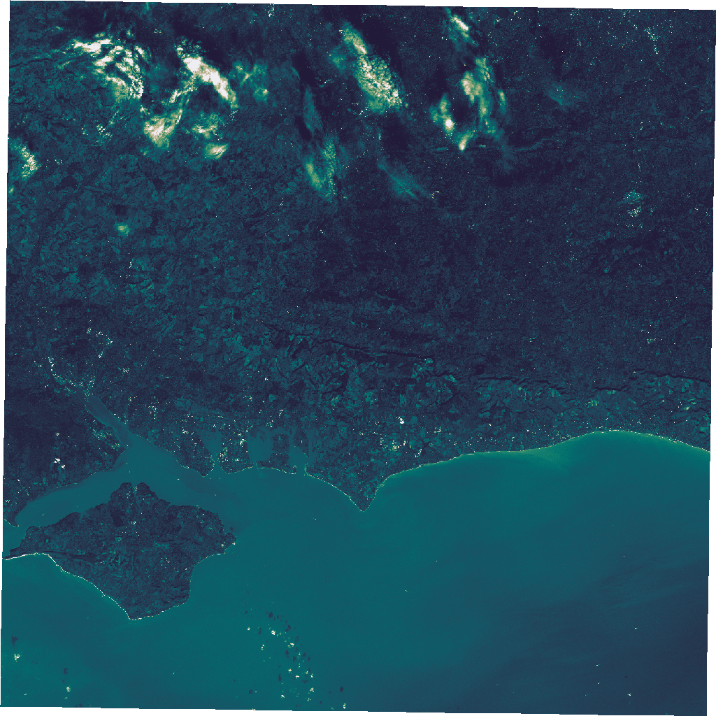

Using Preview with Kerchunk

Lets follow a similar approach for the xarray data. This xarray data is a Kerchunk dataset - remember that it contains a single variable called rsus. We can preview the data similarly to how we previewed the COG data.

This time, focus on the rescale parameter. This parameter is used to rescale the values of the data. In this example we are rescaling between -50,100, but try something new like 50,400 and see how the data changes.

XARRAY_PREVIEW_URL = "https://eodatahub.org.uk/titiler/xarray/tiles/0/0/0"
XARRAY_PARAMS = {
    "url": cmip6_kerchunk_asset.href,
    "variable": "rsus",
    "rescale": "-50,100",
    "colormap_name": "plasma",
    "reference": "true",
}

# Build the request
constructed_url = f"{XARRAY_PREVIEW_URL}?url={cmip6_kerchunk_asset.href}&variable=rsus&rescale=35,400&colormap_name=plasma&reference=true"
print(constructed_url)

# Request the titiler preview
response = requests.get(XARRAY_PREVIEW_URL, params=XARRAY_PARAMS)

# Display the image
image = Image(response.content)
display(image)

https://eodatahub.org.uk/titiler/xarray/tiles/0/0/0?url=https://dap.ceda.ac.uk/badc/cmip6/metadata/kerchunk/pipeline1/ScenarioMIP/THU/CIESM/kr1.0/CMIP6_ScenarioMIP_THU_CIESM_ssp585_r1i1p1f1_Amon_rsus_gr_v20200806_kr1.0.json&variable=rsus&rescale=35,400&colormap_name=plasma&reference=true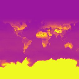

Exploring the Data Using OGC XYZ Tiles

Now that we have previewed the datasets, we can use third party tools to also explore the data. To do this, we are going to create an XYZ tile endpoint for both the COG data and the Kerchunk data. This can then be used in any third-party tool that supports XYZ tiles e.g. QGIS, OpenLayers, Leaflet, etc.

The following code cell builds the URLs we require based on some of the variables that we have already set. It then prints the two URLS that we will need to display andvisualise the data.

# Generate XYZ For COG
COG_OGC_URL = (
    "https://eodatahub.org.uk/titiler/core/cog/tiles/WebMercatorQuad/{z}/{x}/{y}"
)
COG_XYZ = (
    COG_OGC_URL + "?" + "&".join([f"{k}={v}" for k, v in COG_PREVIEW_PARAMS.items()])
)

# Generate XYZ For Xarray
XARRAY_OGC_URL = (
    "https://eodatahub.org.uk/titiler/xarray/tiles/WebMercatorQuad/{z}/{x}/{y}"
)
XARRAY_XYZ = (
    XARRAY_OGC_URL + "?" + "&".join([f"{k}={v}" for k, v in XARRAY_PARAMS.items()])
)

print("Cog XYZ: ", COG_XYZ)
print("Kerchunk XYZ", XARRAY_XYZ)

Cog XYZ:  https://eodatahub.org.uk/titiler/core/cog/tiles/WebMercatorQuad/{z}/{x}/{y}?url=https://dap.ceda.ac.uk/neodc/sentinel_ard/data/sentinel_2/2023/11/17/S2A_20231117_latn509lonw0008_T30UXB_ORB137_20231117131218_utm30n_osgb_vmsk_sharp_rad_srefdem_stdsref.tif&bidx=1&rescale=9,255&colormap_name=rain_r
Kerchunk XYZ https://eodatahub.org.uk/titiler/xarray/tiles/WebMercatorQuad/{z}/{x}/{y}?url=https://dap.ceda.ac.uk/badc/cmip6/metadata/kerchunk/pipeline1/ScenarioMIP/THU/CIESM/kr1.0/CMIP6_ScenarioMIP_THU_CIESM_ssp585_r1i1p1f1_Amon_rsus_gr_v20200806_kr1.0.json&variable=rsus&rescale=-50,100&colormap_name=plasma&reference=true

We can then use a map viewer package such as folium to ingest the titiler URL and display it in an interactive way. We do this below for both datasets.

# For the Sentinel dataset
m = folium.Map(location=[54.5, -4.5], zoom_start=6)

# Add the TiTiler layer
folium.raster_layers.TileLayer(
    tiles=COG_XYZ, attr="TiTiler", name="Sentinel 2 ARD Scene", overlay=True
).add_to(m)

# Add a layer control
folium.LayerControl().add_to(m)

# Display the map
m

Make this Notebook Trusted to load map: File -> Trust Notebook

# For the CMIP6 dataset
m = folium.Map(location=[0, 0], zoom_start=2)

# Add the TiTiler layer
folium.raster_layers.TileLayer(
    tiles=XARRAY_XYZ,
    attr="TiTiler",
    name="CMIP6 Surface Upwelling Shortwave Radiation (W m-2)",
    overlay=True,
).add_to(m)

# Add a layer control
folium.LayerControl().add_to(m)

# Display the map
m

Make this Notebook Trusted to load map: File -> Trust Notebook

In this notebook, we have seen how to access and visualise different data types in different ways.

Extra functionality includes the ability to visualise your own Workspace data by passing in your Workspace API key (that you can generate from the Workspace tab). You can then visualise your own data on a map.

This means you can visualise any of your workflow outputs, commercial data or any other visualisable data you have in your Workspace.

An example request would be:

TITILER_PREVIEW_URL = f'https://eodatahub.org.uk/titiler/core/cog/preview'
TITILER_PREVIEW_PARAMS = {
    'url': WORKFLOW_OUTPUT_ASSET,
    'bidx': 1,
    'rescale': '9,255',
    'colormap_name': 'rain_r'
}

response = requests.get(TITILER_PREVIEW_URL, params=TITILER_PREVIEW_PARAMS, headers={'Authorization': f'Bearer {WORKSPACE_API_KEY}'}) # Note the headers parameter

Here we are passing the WORKSPACE_API_KEY in the headers of the request. This will allow you to visualise your own private data straight from the Platform.