User Example: Temporal Mosaics

Description & purpose: This Notebook introduces the science behind a user example looking to create temporal best pixel temporal mosaics using the Sentinel 2 ARD dataset. It also introduces the EOAP that has been created to run a scaled workflow on EODH.

Author(s): Alastair Graham, Dusan Figala

Date created: 2024-11-08

Date last modified: 2024-11-08

Licence: This file is licensed under Creative Commons Attribution-ShareAlike 4.0 International. Any included code is released using the BSD-2-Clause license.

Copyright (c) , All rights reserved.

Redistribution and use in source and binary forms, with or without modification, are permitted provided that the following conditions are met:

Redistributions of source code must retain the above copyright notice, this list of conditions and the following disclaimer. Redistributions in binary form must reproduce the above copyright notice, this list of conditions and the following disclaimer in the documentation and/or other materials provided with the distribution. THIS SOFTWARE IS PROVIDED BY THE COPYRIGHT HOLDERS AND CONTRIBUTORS “AS IS” AND ANY EXPRESS OR IMPLIED WARRANTIES, INCLUDING, BUT NOT LIMITED TO, THE IMPLIED WARRANTIES OF MERCHANTABILITY AND FITNESS FOR A PARTICULAR PURPOSE ARE DISCLAIMED. IN NO EVENT SHALL THE COPYRIGHT HOLDER OR CONTRIBUTORS BE LIABLE FOR ANY DIRECT, INDIRECT, INCIDENTAL, SPECIAL, EXEMPLARY, OR CONSEQUENTIAL DAMAGES (INCLUDING, BUT NOT LIMITED TO, PROCUREMENT OF SUBSTITUTE GOODS OR SERVICES; LOSS OF USE, DATA, OR PROFITS; OR BUSINESS INTERRUPTION) HOWEVER CAUSED AND ON ANY THEORY OF LIABILITY, WHETHER IN CONTRACT, STRICT LIABILITY, OR TORT (INCLUDING NEGLIGENCE OR OTHERWISE) ARISING IN ANY WAY OUT OF THE USE OF THIS SOFTWARE, EVEN IF ADVISED OF THE POSSIBILITY OF SUCH DAMAGE.

Background

In this example we are required to create a dataset that is cloud-free and temporally mosaiced. The input dataset is to be the CEDA Sentinel 2 ARD image data.

Cloud-free temporal mosaics of optical satellite images are composites created by combining multiple satellite acquisitions over a specific time period to generate a seamless and cloud-free view of a region. Optical satellite imagery, such as data from Sentinel-2, is often obstructed by clouds and atmospheric conditions, limiting the usability of individual acquisitions. Temporal mosaics overcome this challenge by selecting the clearest pixels from a time series of images, typically based on cloud masking algorithms or quality indices. These mosaics preserve spatial and spectral information while minimizing data gaps caused by clouds. Additional methods of data creation include using cloud-masks to remove clouds and/or shadow before the mosaicing step.

A user would want a cloud-free temporal mosaic of Sentinel-2 data to ensure consistent, high-quality imagery for analyzing surface features and environmental changes without the interference of clouds or shadows. Sentinel-2, part of the European Space Agency’s Copernicus program, provides high-resolution optical imagery across 13 spectral bands, making it ideal for applications in agriculture, forestry, urban planning, and climate monitoring. By creating a cloud-free mosaic, users can integrate multiple acquisitions into a single, seamless dataset that eliminates gaps caused by clouds and ensures better temporal and spatial coverage.

Analysis Ready Data (ARD) refers to satellite data that has been pre-processed and formatted to a standardized level, enabling users to perform analysis without needing to conduct significant additional preprocessing. ARD is designed to be easily accessible, interoperable, and suitable for a wide range of scientific and operational applications. The pre-processing typically includes geometric correction, radiometric calibration and atmospheric correction (removing the effects of the atmosphere on reflectance). It may also include cloud masking. The aim of creating ARD is to ensure data is consistent across time and space, and minimise the technical barriers for users, allowing them to focus on extracting insights rather than preparing raw data. By eliminating much of the preprocessing workload, ARD democratises the use of satellite data, allowing non-specialists and researchers to use the data more efficiently and reliably.

Such temporal mosaics are particularly valuable for applications requiring reliable, large-area analysis. For example, in agriculture, a cloud-free mosaic allows precise monitoring of crop health, phenological changes, and yield estimation by preserving uninterrupted vegetation indices. In forestry, it supports accurate assessments of deforestation, canopy density, and biomass. For urban planning and disaster management, cloud-free mosaics provide unobstructed views of land use changes, infrastructure, and affected regions, critical for decision-making.

The Scientific Process

Before creating a workflow on the EODH platform it was important to step through the scientific process to make sure that the correct tools and data were being considered.

To create the cloud-free outputs we use the cloud mask supplied with the ARD dataset. The information held in the cloud mask layer is used to block out the existing areas of cloud, and is applied to every band.

The temporal mosaic is created using a command line set of tools called pktools. Although a slightly older set of tools it is incredibly versatile, and being command-line first lends itself to the EOAP/CWl way of working. One of the tools, pkcomposite, is used to generate a median image from all input images over a one month period.

Processing steps

• pyeodh search of sentinel2_ard STAC (inputs are an AOI polygon (we need this later) and a date range)
• STEP 1: for each band in each returned image apply the cloud mask to remove cloud pixels from the data
  • this results in a multibanded image that is cloud-masked
  • need to retain information on original image capture date
  • output should be a temporary STAC catalog
• STEP 2: for each cloud-masked image in a given month create band composites cropped to the AOI
  • e.g. pkcomposite -i in_A.tif -i in_B.tif -i in_C.tif -o out_b1.tif -cr median -b 0 -e aoi.geojson
  • need to be able to supply all images, the aoi polygon, and the composite method (e.g. median)
  • output should be a STAC catalog of spatially cropped single-band composites for each month (e.g. for a three month period and 4 band input data there should be 3x Band1 outputs, 3x Band2 outputs, 3x Band3 outputs, 3x Band4 outputs)

The following tutorial demonstrates how to process data held in the Sentinel S2 ARD STAC.

Scientific method

First we need to import the required packages.

import pyeodh
import xarray as xr
import rioxarray
import os
from pathlib import Path
import requests
import threading

# set the area of interest

thetford_aoi = {
    "coordinates": [
        [
            [0.08905898091569497, 52.69722175598818],
            [0.08905898091569497, 52.15527412683906],
            [0.9565339502005088, 52.15527412683906],
            [0.9565339502005088, 52.69722175598818],
            [0.08905898091569497, 52.69722175598818],
        ]
    ],
    "type": "Polygon",
}

Next we need to connect to the resource catalogue and undertake a search of the sentinel2_ard catalogue for the AOI location within a specific date range

# connect to 
rc = pyeodh.Client().get_catalog_service()

items = rc.search(
    collections=["sentinel2_ard"],
    catalog_paths=["supported-datasets/ceda-stac-catalogue"],
    intersects=thetford_aoi,
    query=[
        "start_datetime>=2023-04-01",
        "end_datetime<=2023-06-30",
    ],
    limit=1,
)

Next, for each item open the cog, cloud and valid .tif assets and download them if needed.

for item in items.get_limited()[0:1]:
    cloud_href = item.assets["cloud"].href
    valid_href = item.assets["valid_pixels"].href
    cog_href = item.assets["cog"].href
    item
    print(item.id, cloud_href, valid_href, cog_href, sep="\n")
    valid = rioxarray.open_rasterio(
        valid_href,
        chunks=True,
    )
    cloud = rioxarray.open_rasterio(
        cloud_href,
        chunks=True,
    )

    # Check if cog file exists locally, if not download it
    cog_filename = f"data/{Path(cog_href).name}"
    if not os.path.isfile(cog_filename):
        with requests.get(cog_href, stream=True) as r:
            r.raise_for_status()
            with open(cog_filename, "wb") as f:
                for chunk in r.iter_content(chunk_size=8192):
                    f.write(chunk)

    cog = rioxarray.open_rasterio(cog_filename, chunks=True)
    print("==" * 10)
    print("success")
    break

The next steps are to create a definitive mask using the amalgamation of the valid pixels layer and the cloud mask layer.

result = valid + cloud

# Set values greater than 1 to 0, others remain as 1
result = xr.where(result > 1, 0, 1)

If we now multiply the cloud optimised geotif file by the result maskfile, expanded to match the shape of cog then each of the bands will have the clouds removed. This is a brute force approach for the purposes of generating a demonstrable workflow and in an operational context a user would likely want to undertand the impact of cloud in individual bands and use specific methods to remove that.

Finally the output is saved to a file

# Multiply cog.tif by the result
# We need to expand the result to match the shape of cog
fin = cog * result.squeeze("band").expand_dims(band=cog.band)

# save to a file
fin.rio.to_raster(raster_path=f"data/rm_cloud.tif", tiled=True, lock=threading.Lock())

As mentioned, one method of generating the composite is to use pktools. It’s an older code, but it checks out. An alternative using Python might be to use xarray and the functions within that package. pktools works well for this use case as the command can be inserted directly

https://pktools.nongnu.org/html/pkcomposite.html

Outputs

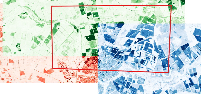
The following images provide an indication of how the pkcomposite tool works. The first image shows three input images (single band in this instance, coloured red, green and blue for clarity) that overlap a specific area of interest. The AOI is marked by the red boundary.

The second image plots the result of the pkcomposite command over the top. It shows how a median layer is created within the bounding box of the AOI.

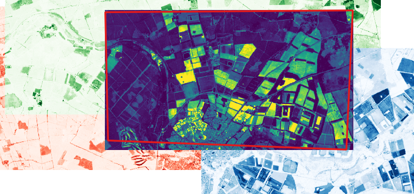
In an EOAP cointext this could be scaled up across multiple multi-band images for a larger AOI.

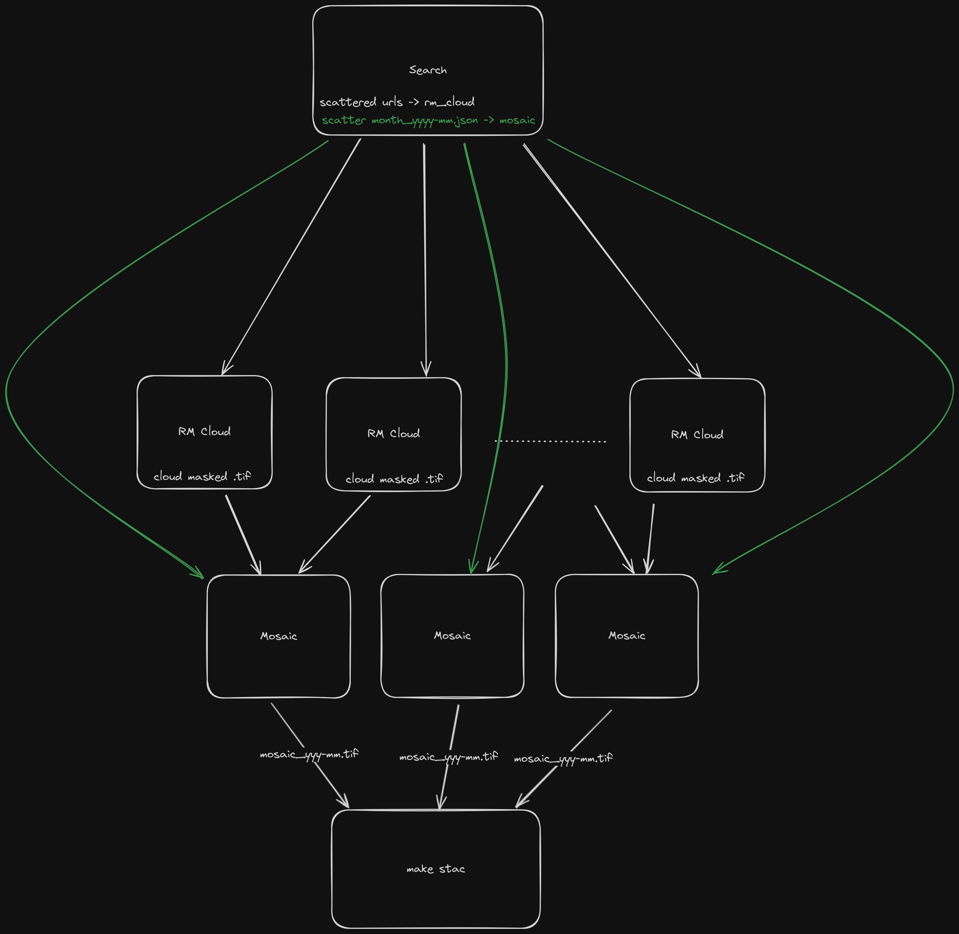
Generating the workflow

We can use eoap-gen to create a suitable workflow for this methodology. The first thing to do is understand the steps and the flow of data through the EODH workflow runner. The following diagram demonstrates how images are searched for and then scattered across numerous processing nodes to remove the cloud. The cloud-free images are then returned to fewer nodes to be mosaiced by month. Finally the mosaics are written out to a searchable STAC directory.

Cloudfree Workflow

Using the configuration file here and reproduced below, it is possible to run eoap-gen to create the full package requirements.

id: cloud-free-best-pixel
doc: Generate cloud free best pixel mosaic on a per month basis
label: Cloud free best pixel

resources: # current ADES max is 4 cores and 16GB RAM, we need all we can get
  cores_min: 4
  ram_min: 16000

inputs:
  - id: catalog
    label: Catalog path
    doc: Full catalog path
    type: string
    default: supported-datasets/ceda-stac-catalogue
  - id: collection
    label: collection id
    doc: collection id
    type: string
    default: sentinel2_ard
  - id: intersects
    label: Intersects
    doc: >
      a GeoJSON-like json string, which provides a "type" member describing the type of the geometry and "coordinates" 
      member providing a list of coordinates. Will search for images intersecting this geometry.
    type: string
    default: >
      {
        "type": "Polygon",
        "coordinates": [
          [
            [0.08905898091569497, 52.69722175598818],
            [0.08905898091569497, 52.15527412683906],
            [0.9565339502005088, 52.15527412683906],
            [0.9565339502005088, 52.69722175598818],
            [0.08905898091569497, 52.69722175598818]
          ]
        ]
      }
  - id: start_datetime
    label: Start datetime
    doc: Start datetime
    type: string
    default: "2023-04-01"
  - id: end_datetime
    label: End datetime
    doc: End datetime
    type: string
    default: "2023-06-30"

outputs:
  - id: stac_output
    type: Directory
    source: s2_make_stac/stac_catalog
steps:
  - id: s2_search
    script: S2-cloud-free-best-pixel/cli/search/search.py
    requirements: S2-cloud-free-best-pixel/cli/search/requirements.txt
    inputs:
      - id: catalog
        source: cloud-free-best-pixel/catalog
      - id: collection
        source: cloud-free-best-pixel/collection
      - id: intersects
        source: cloud-free-best-pixel/intersects
      - id: start_datetime
        source: cloud-free-best-pixel/start_datetime
      - id: end_datetime
        source: cloud-free-best-pixel/end_datetime
    outputs:
      - id: urls
        type: string[]
        outputBinding:
          loadContents: true
          glob: urls.txt
          outputEval: $(self[0].contents.split('\n'))
      - id: months
        type: File[]
        outputBinding:
          glob: month_*.json

  - id: s2_rm_cloud
    script: S2-cloud-free-best-pixel/cli/rm_cloud/rm_cloud.py
    requirements: S2-cloud-free-best-pixel/cli/rm_cloud/requirements.txt
    conda:
      - dask
      - gdal
    scatter_method: dotproduct
    inputs:
      - id: item_url
        source: s2_search/urls
        scatter: true
    outputs:
      - id: cloud_masked
        type: File
        outputBinding:
          glob: "*.tif"

  - id: s2_mosaic
    script: S2-cloud-free-best-pixel/cli/mosaic/mosaic.py
    requirements: S2-cloud-free-best-pixel/cli/mosaic/requirements.txt
    apt_install:
      - pktools
    scatter_method: dotproduct
    inputs:
      - id: intersects
        source: cloud-free-best-pixel/intersects
      - id: month_json
        source: s2_search/months
        scatter: true
        type: File
      - id: all_images
        source: s2_rm_cloud/cloud_masked
        type: File[]
    outputs:
      - id: best_pixel
        type: File
        outputBinding:
          glob: "*.tif"

  - id: s2_make_stac
    script: S2-cloud-free-best-pixel/cli/make_stac/make_stac.py
    requirements: S2-cloud-free-best-pixel/cli/make_stac/requirements.txt
    inputs:
      - id: geometry
        source: cloud-free-best-pixel/intersects
      - id: files
        source: s2_mosaic/best_pixel
        type: File[]
    outputs:
      - id: stac_catalog
        outputBinding:
          glob: .
        type: Directory

Running the configuration file results in the directory available here which can then be submitted to EODH using pyeodh and run using either the API client or QGIS plugin.